1D setups
Advection (1D)
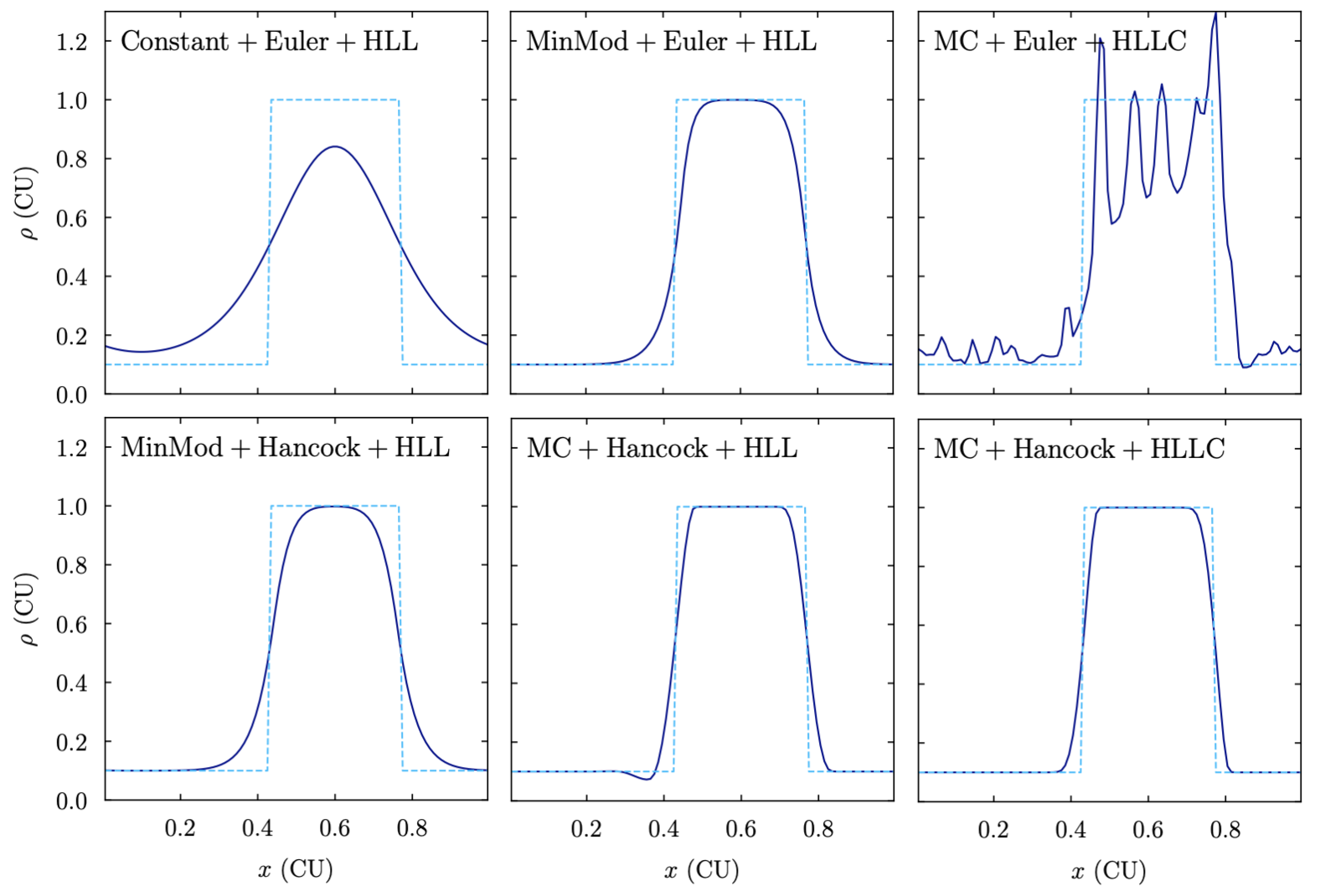
The image below shows how different hydro algorithms perform (or fail) at advecting a tophat density across the domain:
- class ulula.setups.advection_1d.SetupAdvection1D(shape='sine', unit_l=1.0, unit_t=1.0, unit_m=1.0)
1D advection test
This setup represents the perhaps simplest meaningful test of a hydro solver. An initial distribution in density is advected at a constant velocity across the domain. The shape should be preserved. This setup demonstrates
Stability and instability of schemes
Importance of choices such as slope limiters and Riemann solvers.
- Parameters:
- shape: str
Initial density shape that is being advected. Can be
'sine'or'tophat'.- unit_l: float
Code unit for length in units of centimeters.
- unit_t: float
Code unit for time in units of seconds.
- unit_m: float
Code unit for mass in units of gram.
- __init__(shape='sine', unit_l=1.0, unit_t=1.0, unit_m=1.0)
Soundwave
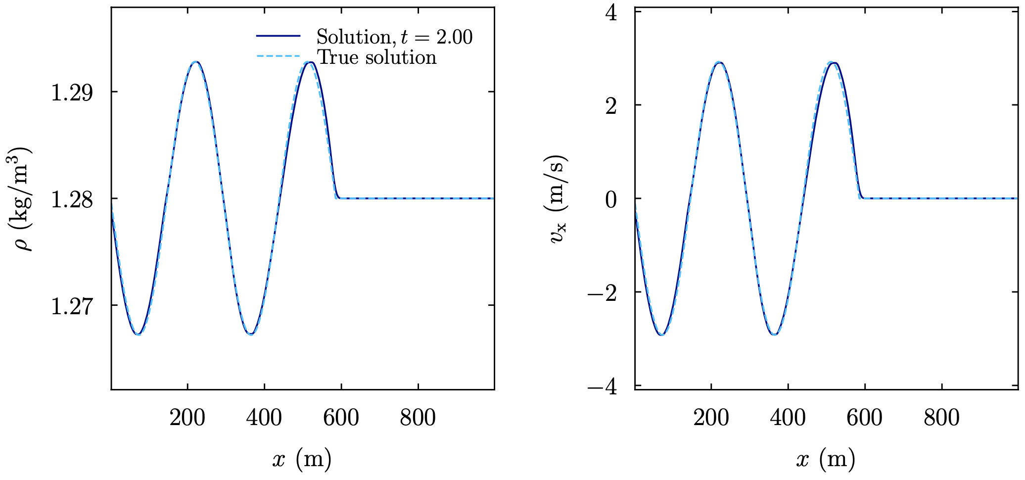
The image below shows how a sound wave travels from the left edge across the domain:
- class ulula.setups.soundwave.SetupSoundwave(L=100000.0, frequency=1.0, amplitude=0.01, eos_mode='ideal', eos_T_K=300.0, unit_l=100000.0, unit_t=1.0, unit_m=1000000000000.0)
Propagating sound wave
A sound wave is created at the left edge of the domain and travels to the right. We assume the density and adiabatic index of air, and either standard pressure or an isothermal EOS given by a particular temperature. This setup demonstrates
User-defined boundary conditions on one side of the domain
Outflow boundary conditions on another side
Difference between ideal and isothermal equations of state
Code units.
The true solution is based on linear theory, which only holds for small amplitudes. We observe wave steepening for large amplitudes.
- Parameters:
- L: float
The box size in cm.
- frequency: float
The frequency of the soundwave in Hertz.
- amplitude: float
The relative amplitude by which the density oscillates compared to the background.
- eos_mode: str
Can be
'ideal'or'isothermal'.- eos_T_K: float
Air temperature in Kelvin (if using isothermal EOS, ignored otherwise).
- unit_l: float
Code unit for length in units of centimeters.
- unit_t: float
Code unit for time in units of seconds.
- unit_m: float
Code unit for mass in units of gram.
- __init__(L=100000.0, frequency=1.0, amplitude=0.01, eos_mode='ideal', eos_T_K=300.0, unit_l=100000.0, unit_t=1.0, unit_m=1000000000000.0)
Shocktube
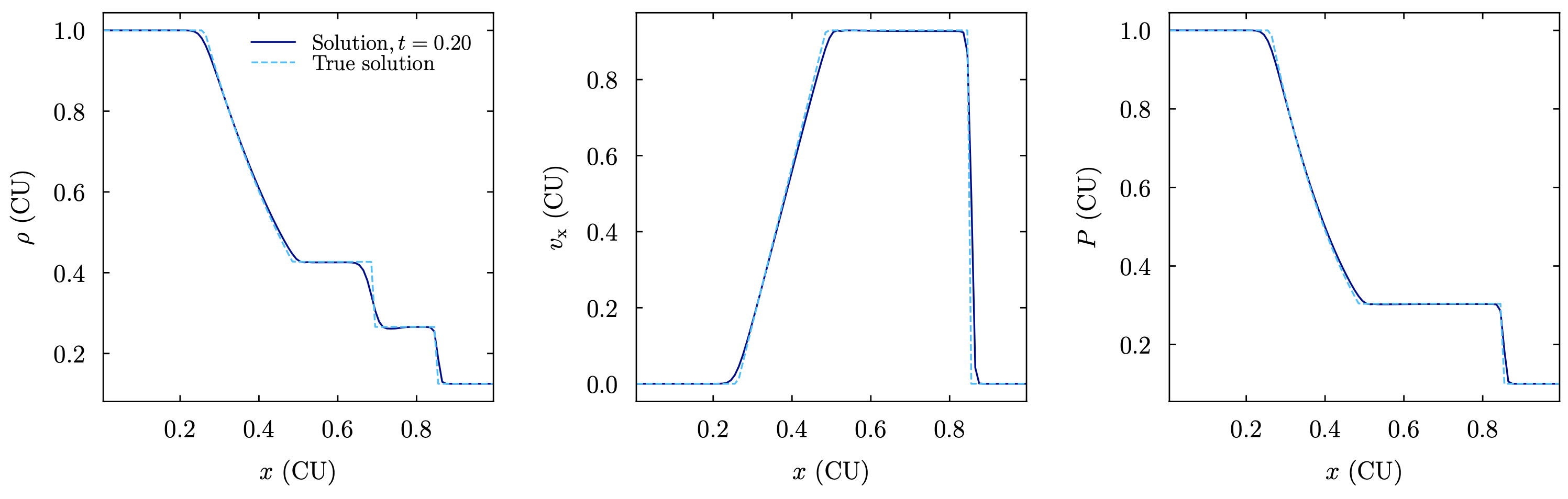
The image below shows the shocktube test for the default hydro solver:
- class ulula.setups.shocktube.SetupShocktube(gamma=1.4, x0=0.5, rhoL=1.0, rhoR=0.125, PL=1.0, PR=0.1, vL=0.0, vR=0.0, unit_l=1.0, unit_t=1.0, unit_m=1.0)
Shocktube problem
The shocktube setup represents a Riemann problem, i.e., a sharp discontinuity in a 1D domain. The default parameters represent the Sod (1978) setup, which is a classic test for Riemann solvers. The sharp break in fluid properties causes a shock and a contact discontinuity traveling to the right and a rarefaction wave traveling to the left. This setup demonstrates:
Ability of hydro solver to handle strong shocks
Impact of slope limiting on the solution
Softening of sharp discontinuities at lower resolution.
The Sod problem can be solved analytically. The solution used here is based on lecture notes by Frank van den Bosch (pdf) and Susanne Hoefner (pdf). However, this solution may not work for all sets of input parameters.
- Parameters:
- gamma: float
The adiabatic index of the ideal gas.
- x0: float
The position of the discontinuity.
- rhoL: float
The density of the left state.
- rhoR: float
The density of the right state.
- PL: float
The pressure of the left state.
- PR: float
The pressure of the right state.
- vL: float
The velocity of the left state.
- vR: float
The velocity of the right state.
- unit_l: float
Code unit for length in units of centimeters.
- unit_t: float
Code unit for time in units of seconds.
- unit_m: float
Code unit for mass in units of gram.
- __init__(gamma=1.4, x0=0.5, rhoL=1.0, rhoR=0.125, PL=1.0, PR=0.1, vL=0.0, vR=0.0, unit_l=1.0, unit_t=1.0, unit_m=1.0)
Free-fall
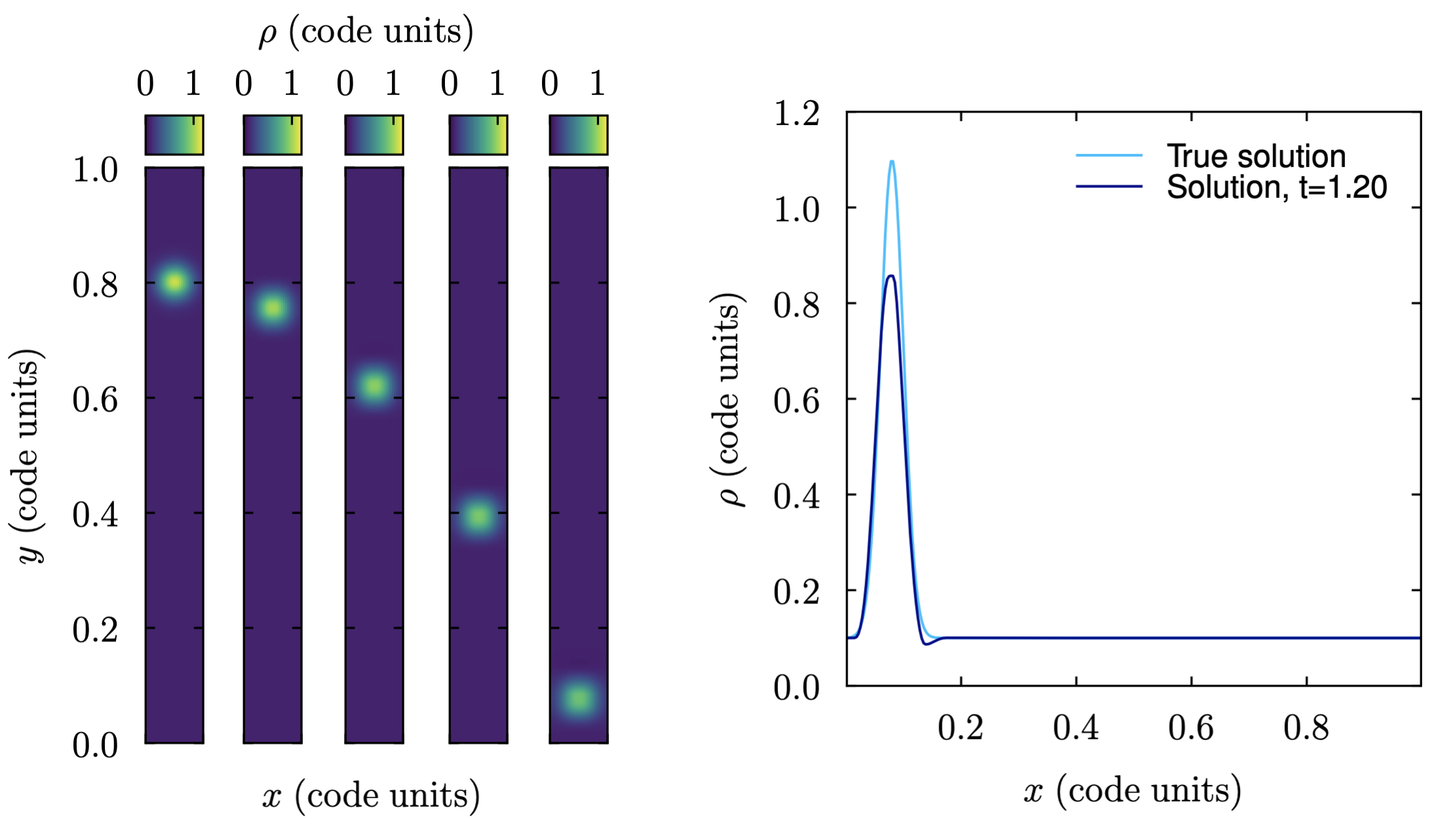
The image below shows the free-fall test at the initial and two later times:
- class ulula.setups.freefall.SetupFreefall(unit_l=1.0, unit_t=1.0, unit_m=1.0)
Gravitational free-fall
This setup is mostly a test of the gravity solver. The outflow BCs mean that the entire domain is free-falling under a constant gravitational acceleration. We compare the position of a Gaussian gas blob in pressure equilibrium to the known solution. This setup demonstrates
Fixed-acceleration gravity combined with outflow boundary conditions
Accuracy of the gravity source term.
- Parameters:
- unit_l: float
Code unit for length in units of centimeters.
- unit_t: float
Code unit for time in units of seconds.
- unit_m: float
Code unit for mass in units of gram.
- __init__(unit_l=1.0, unit_t=1.0, unit_m=1.0)
Atmosphere
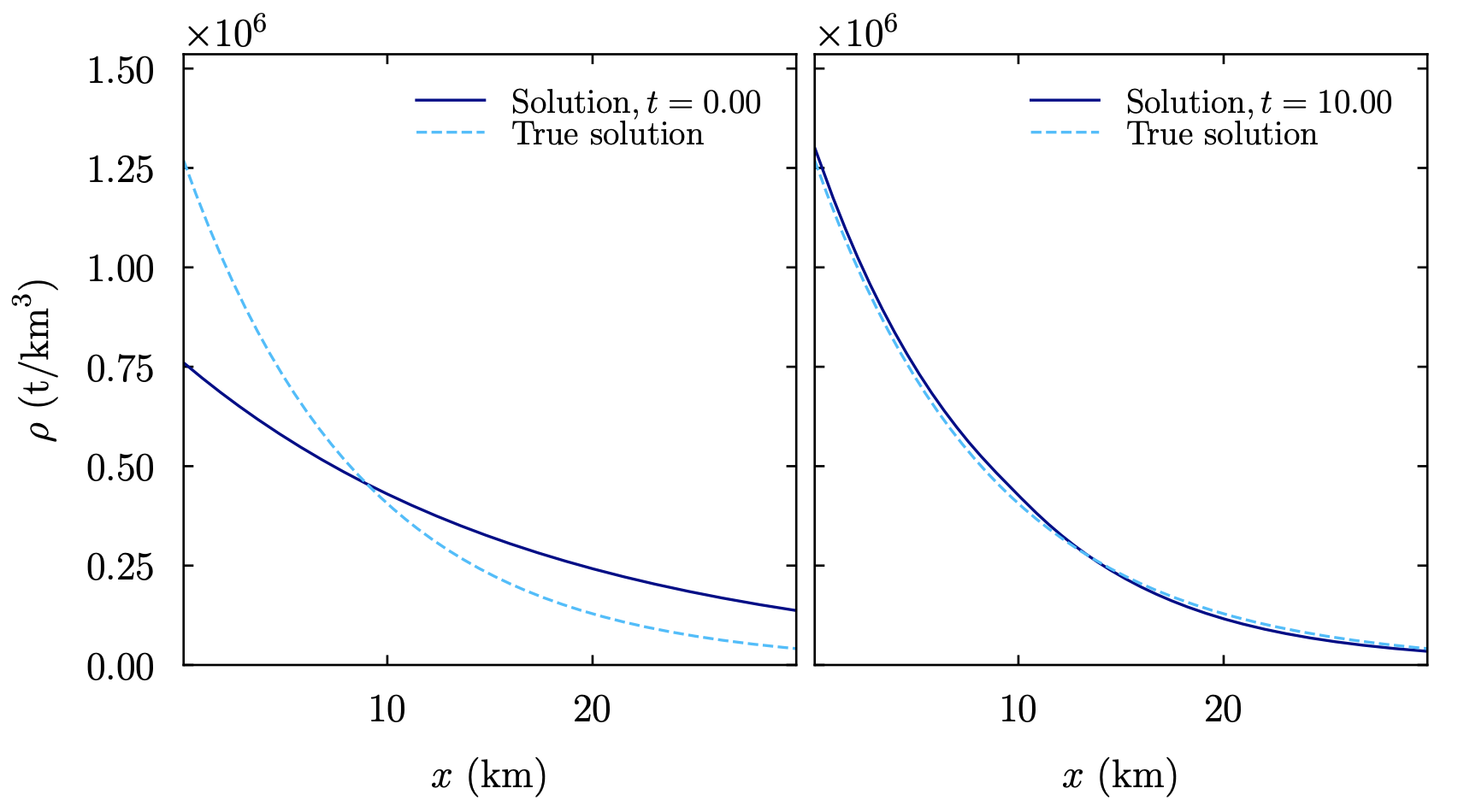
The image below shows the atmosphere setup at the initial time and after 10 hours:
- class ulula.setups.atmosphere.SetupAtmosphere(eos_mode='isothermal', T=270.0, xmax=30.0, unit_l=100000.0, unit_t=3600.0, unit_m=1000000000000.0)
Earth’s hydrostratic atmosphere
This setup represents the Earth’s atmosphere in 1D. This hydro problem can be solved analytically for a fixed temperature, but in reality the temperature does evolve somewhat with altitude. This setup thus offers two modes. For an isothermal EOS, the air settles into an exponential density and pressure profile. We perturb the initial density away from the known solution by assuming a “wrong” scale height. After some time, the atmosphere settles to the correct solution.
If the ideal gas EOS is chosen, a piecewise-linear approximation to the known temperature profile is enforced at each timestep. In this setup, the initial profile is set to the isothermal solution, and that solution is also plotted as the “true solution” for comparison. This setup demonstrates
Fixed-acceleration gravity with wall boundary conditions
Isothermal and ideal equations of state
Code units suitable to Earth conditions, including Earth gravity
User-defined function to update the fluid state at runtime.
By default, the code units are set to kilometers, hours, and tons. Depending on the initial conditions, the setup can be numerically unstable due to strong motions that develop into shocks. For example, if too much mass is initially placed in the upper atmosphere, that mass falls to the surface. Similarly, extending the upper limit to much higher altitude than the default of 30 km can lead to difficulties due to the very low pressure and density.
- Parameters:
- eos_mode: str
Equation of state to use. Can be
'isothermal', in which case the temperature is set by theTparameter, or'ideal', in which case an approximation to Earth’s true atmosphere used.- T: float
Air temperature in Kelvin for isothermal equation of state; ignored for ideal gas EOS.
- xmax: float
The height of the domain in code units (kilometers by default). This number cannot get arbitrarily large because the density and pressure get very low, which can lead to numerical instabilities.
- unit_l: float
Code unit for length in units of centimeters.
- unit_t: float
Code unit for time in units of seconds.
- unit_m: float
Code unit for mass in units of gram.
- __init__(eos_mode='isothermal', T=270.0, xmax=30.0, unit_l=100000.0, unit_t=3600.0, unit_m=1000000000000.0)
Jeans instability
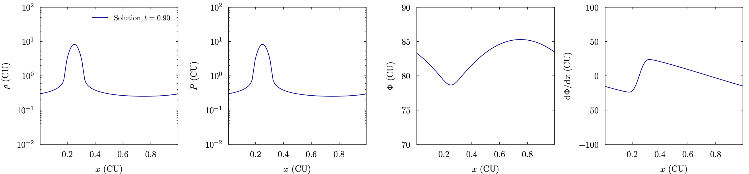
The image below shows the Jeans instability setup as the perturbation is collapsing:
- class ulula.setups.jeans_instability.SetupJeansInstability(lam=1.0, lam_J=1.3, amplitude=0.01, unit_l=1.0, unit_t=1.0, unit_m=1.0)
Jeans instability
In this setup, a background state with constant density and (isothermal) pressure is perturbed by a sine wave. Depending on the ratio of the wavenumber to the critical “Jeans wavenumber,” the perturbation is stable (if \(\lambda < \lambda_{\rm J}\), meaning the fluid state oscillates) or unstable (if \(\lambda > \lambda_{\rm J}\), meaning the perturbation collapses). In practice, we seem to need \(\lambda_{\rm J} / \lambda \sim 1.5\) for stability. This setup demonstrates
Self-gravity and run-away collapse
Stability criteria.
- Parameters:
- lam: float
The wavelength of the initial perturbation, where unity corresponds to one wave across the domain.
- lam_J: float
The critical Jeans wavelength for stability, which is determined by the balance between pressure and gravity. We set the gravitational constant according to this number.
- amplitude: float
The amplitude of the initial perturbation as a fraction of the background density.
- unit_l: float
Code unit for length in units of centimeters.
- unit_t: float
Code unit for time in units of seconds.
- unit_m: float
Code unit for mass in units of gram.
- __init__(lam=1.0, lam_J=1.3, amplitude=0.01, unit_l=1.0, unit_t=1.0, unit_m=1.0)