2D setups
Advection (2D)
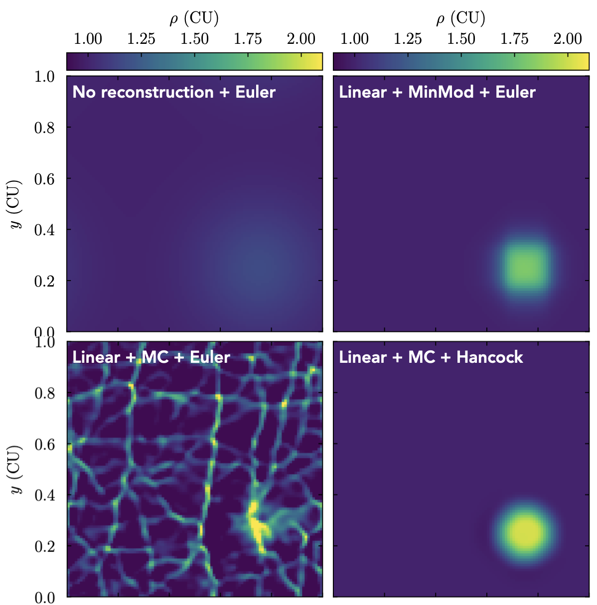
The following image shows how different hydro algorithms perform (or fail) in the 2D advection test:
- class ulula.setups.advection_2d.SetupAdvection2D(shape='tophat', unit_l=1.0, unit_t=1.0, unit_m=1.0)
2D advection test
In this test, an initially overdense tophat or sine pattern is placed at the center of the domain. The entire fluid moves towards the northeast direction. The edges of the disk diffuse into the surrounding fluid at a rate that depends on the hydro solver. For example, when using no spatial reconstruction, the hydro scheme will be extremely diffusive and the tophat will quickly spread into the surrounding fluid. Linear interpolation leads to less diffusion, especially if an aggressive slope limiter is used. However, when combining the resulting sharp gradients with a hydro scheme that is 1st-order in time, the test quickly becomes unstable and fails spectacularly. This setup demonstrates
Stability of time integration schemes
Diffusivity of reconstruction schemes
Importance of slope limiters.
- Parameters:
- shape: str
Initial shape of density that is being advected. Can be
'sine'or'tophat'.- unit_l: float
Code unit for length in units of centimeters.
- unit_t: float
Code unit for time in units of seconds.
- unit_m: float
Code unit for mass in units of gram.
- __init__(shape='tophat', unit_l=1.0, unit_t=1.0, unit_m=1.0)
Kelvin-Helmholtz instability
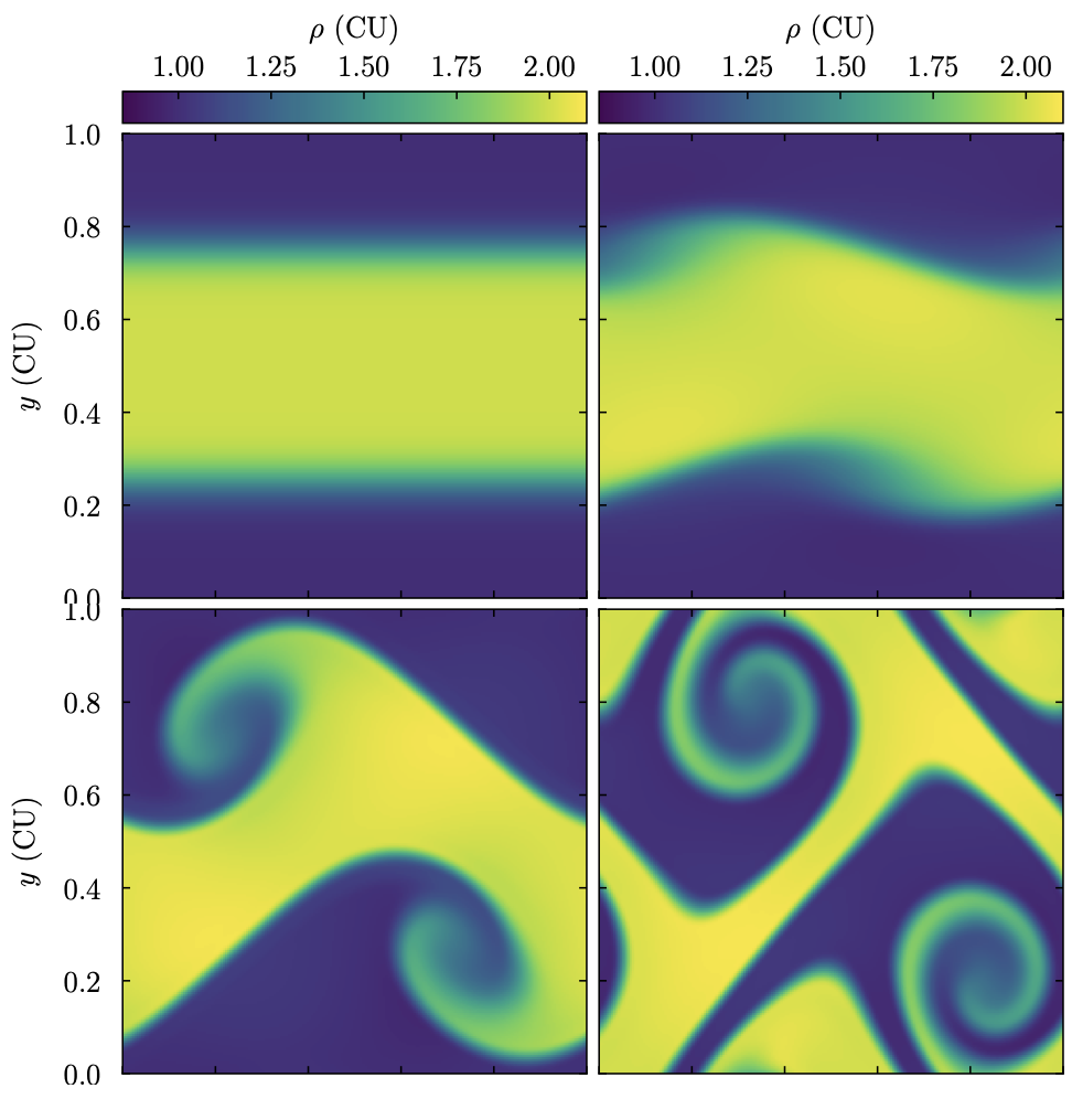
The following image shows the evolution of density in the Kelvin-Helmholtz setup:
- class ulula.setups.kelvin_helmholtz.SetupKelvinHelmholtz(sharp_ics=False, n_waves=1, unit_l=1.0, unit_t=1.0, unit_m=1.0)
Kelvin-Helmholtz instability
The KH instability forms at the interface between two fluids that are moving past each other. The user can choose between a setup where the interface is infinitely sharp and the smooth ICs of Robertson et al. 2010. In the sharp case, the instability is seeded by grid noise, but we still add a small velocity perturbation to obtain more well-defined behavior. The smooth version is recommended as it leads to a more physical test case. This setup demonstrates
Instability at two-fluid interface
Periodic boundary conditions
Sharp vs. smooth gradients in initial conditions.
- Parameters:
- sharp_ics: bool
Use sharp boundary between fluids instead of smoothed ICs.
- n_waves: int
Number of wave periods in the domain. The number of periods that can be resolved depends on the resolution.
- unit_l: float
Code unit for length in units of centimeters.
- unit_t: float
Code unit for time in units of seconds.
- unit_m: float
Code unit for mass in units of gram.
- __init__(sharp_ics=False, n_waves=1, unit_l=1.0, unit_t=1.0, unit_m=1.0)
Cloud crushing
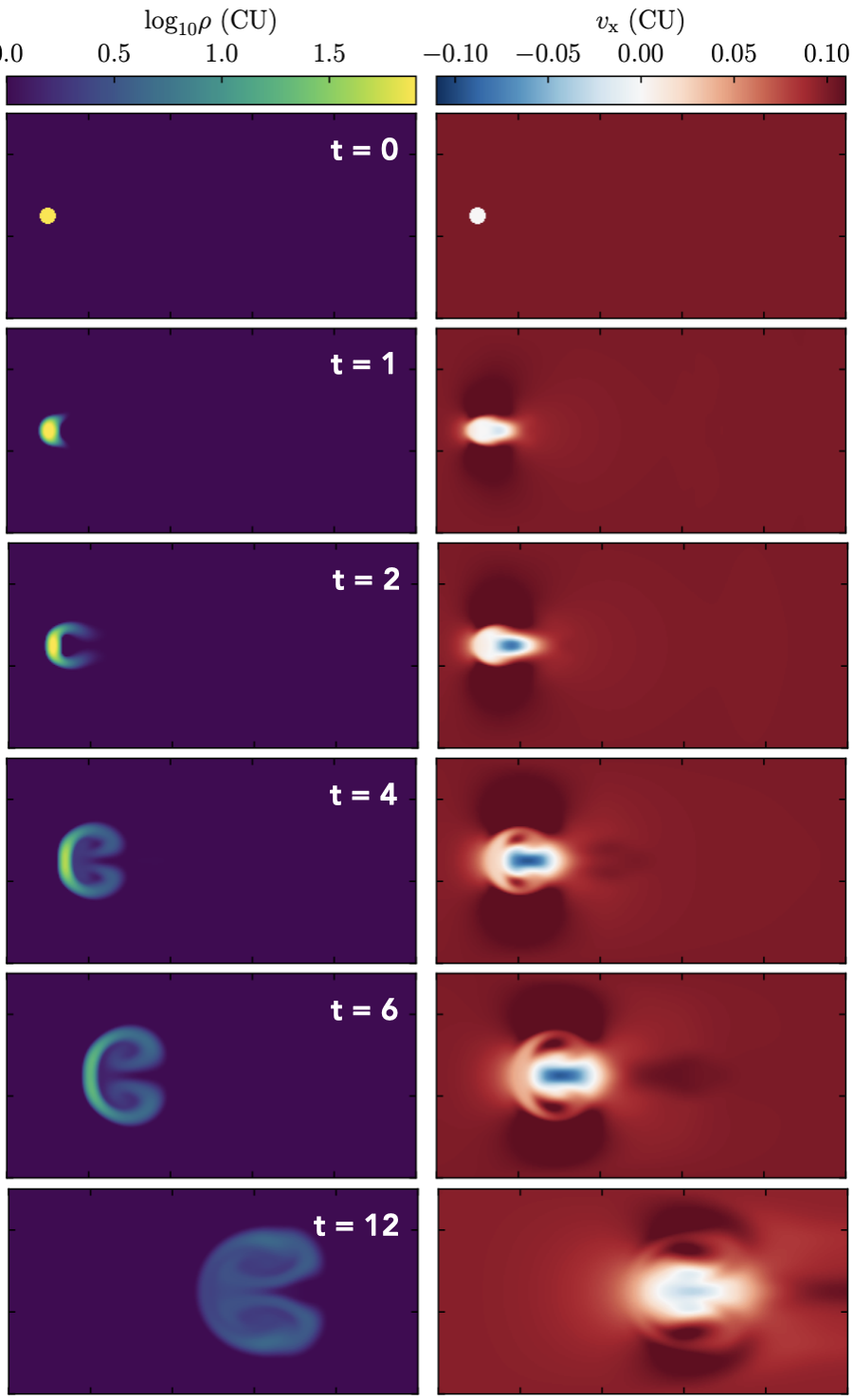
The following image shows the evolution of density and x-velocity in the cloud crushing setup:
- class ulula.setups.cloud_crushing.SetupCloudCrushing(unit_l=1.0, unit_t=1.0, unit_m=1.0)
Cloud-crushing setup
In this classic setup, a dense cloud is embedded in a hot, fast-moving, less dense wind at equal pressure. The sharp cloud edge creates some initial shocks, but those quicky leave the domain given the outflow boundary conditions. The cloud is rapidly destroyed, but the rate of destruction and the details of the evolution depend quite strongly on resolution. It is tempting to simply set outflow boundary conditions, but the fluid can back-react on the left edge as the flow is reflected off the dense blob. Thus, we manually enforce the wind state in the left boundary. This setup demonstrates
Rectangular domain shapes
Mixture of standard and user-defined boundary conditions
Strong resolution dependence.
- Parameters:
- unit_l: float
Code unit for length in units of centimeters.
- unit_t: float
Code unit for time in units of seconds.
- unit_m: float
Code unit for mass in units of gram.
- __init__(unit_l=1.0, unit_t=1.0, unit_m=1.0)
Sedov-Taylor explosion
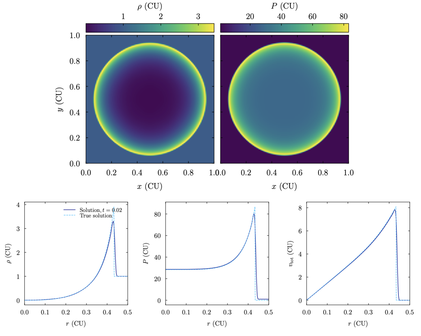
The following image shows the Sedov-Taylor blastwave setup as the shock is about to reach the edge of the domain, plotted both in 2D and 1D:
- class ulula.setups.sedov_taylor.SetupSedovTaylor(E=50.0, rho0=1.0, gamma=1.6666666666666667, unit_l=1.0, unit_t=1.0, unit_m=1.0)
Sedov-Taylor explosion
The Sedov-Taylor solution represents a blastwave created by a large amount of energy that is injected at the center of the domain. In this setup, the energy is distributed in a Gaussian with a radius of ~1 cell. which avoids grid artifacts that can arise to the square nature of the cells. If the energy is much larger than the thermal energy of the surrounding gas, the solution is self-similar, i.e., does not depend on any physical scale and evolves in time as a power-law. The exact solution is adapted from the Gandalf code by Hubber et al. (2018). This setup demonstrates
Radial 1D plotting through a 2D domain
Accuracy of the propagation of a strong shock.
- Parameters:
- E: float
Explosion energy in code units. The thermal energy in the domain is about unity in these units, so
Eshould be significantly larger than unity.- rho0: float
The density of the surrounding medium in code units.
- gamma: float
The adiabatic index of the gas.
- unit_l: float
Code unit for length in units of centimeters.
- unit_t: float
Code unit for time in units of seconds.
- unit_m: float
Code unit for mass in units of gram.
- __init__(E=50.0, rho0=1.0, gamma=1.6666666666666667, unit_l=1.0, unit_t=1.0, unit_m=1.0)
Gresho Vortex
The following image shows the Gresho vortex setup after a number of revolutions, plotted both in 2D and 1D:
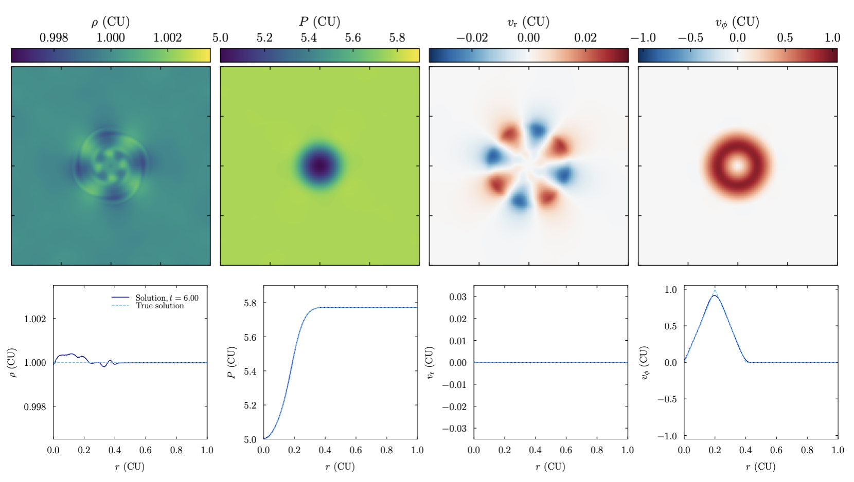
- class ulula.setups.gresho_vortex.SetupGreshoVortex(unit_l=1.0, unit_t=1.0, unit_m=1.0)
Gresho Vortex
This setup tests the symmetry and angular momentum conservation of the hydro solver. A ring at the center of the domain has positive azimuthal velocity, which creates a centrifugal force that is balanced by pressure gradients. Ideally, the setup should be stable as the gas rotates around the center. Any smoothing of the ring is an indication that angular momentum is not perfectly preserved. The problem was presented in Gresho & Sani 1987 (see also Liska & Wendroff 2003). This setup demonstrates
Computing and plotting of azimuthal velocities
Angular momentum conservation.
- Parameters:
- unit_l: float
Code unit for length in units of centimeters.
- unit_t: float
Code unit for time in units of seconds.
- unit_m: float
Code unit for mass in units of gram.
- __init__(unit_l=1.0, unit_t=1.0, unit_m=1.0)
Rayleigh-Taylor instability
The following image shows the evolution of density the Rayleigh-Taylor instability setup:
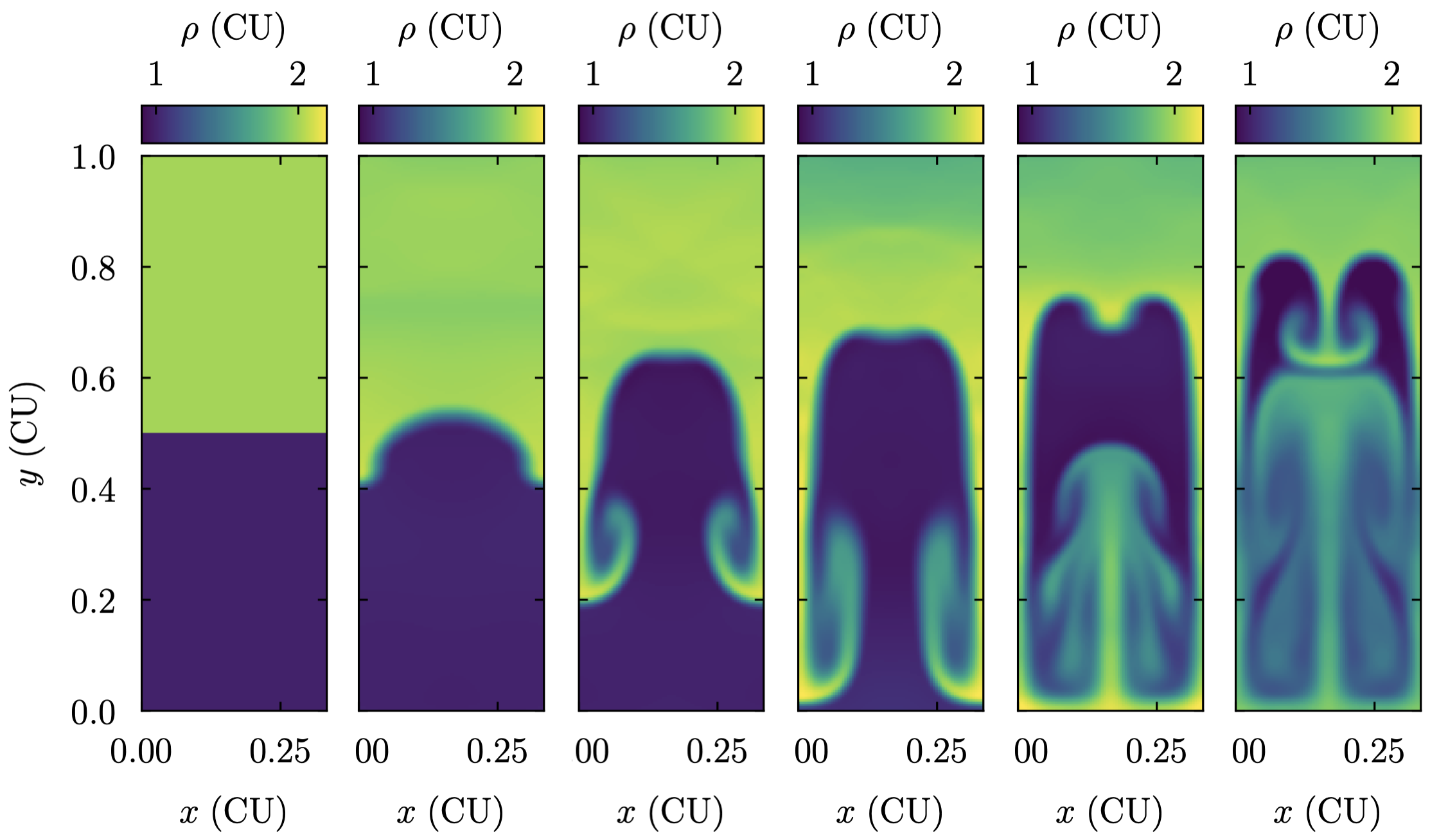
- class ulula.setups.rayleigh_taylor.SetupRayleighTaylor(aspect_ratio=3.0, amplitude=0.1, frequency=0.5, phase=0.0, amplitude_2=0.0, frequency_2=0.0, phase_2=0.0, unit_l=1.0, unit_t=1.0, unit_m=1.0)
Rayleigh-Taylor instability
In this well-known setup, a denser fluid sits on top of a less dense fluid. As the boundary is perturbed with a small velocity, a mushroom-like structure forms. The default setup corresponds to a single peak in velocity at the center of the center of the domain, but the user can investigate multiple linearly added perturbations as well. This setup demonstrates:
Fixed-acceleration gravity in 2D with wall boundary conditions
Instabilities at a two-fluid interface, including their dependence on the scale of perturbations.
- Parameters:
- aspect_ratio: float
The ratio of y to x extent of the domain.
- amplitude: float
The amplitude of the initial y-velocity at the interface.
- frequency: float
The number of sine wave periods by which the boundary between fluids is perturbed. Unity corresponds to one full wave across the x-range of the domain, one-half corresponds to a single wave peak.
- phase: float
A phase to add to the sine wave argument, where unity corresponds to a shift by a full wavelength (\(2 \pi\) radians).
- amplitude_2: float
Like
amplitude, but for a second wave that can optionally be added on top of the first to study the behavior of the RT instability for different perturbations.- frequency_2: float
Like
frequencybut for the second wave.- phase_2: float
Like
phasebut for the second wave.- unit_l: float
Code unit for length in units of centimeters.
- unit_t: float
Code unit for time in units of seconds.
- unit_m: float
Code unit for mass in units of gram.
- __init__(aspect_ratio=3.0, amplitude=0.1, frequency=0.5, phase=0.0, amplitude_2=0.0, frequency_2=0.0, phase_2=0.0, unit_l=1.0, unit_t=1.0, unit_m=1.0)
Tidal disruption
The following image shows the gravitational potential and the density evolution of the tidal disruption setup:
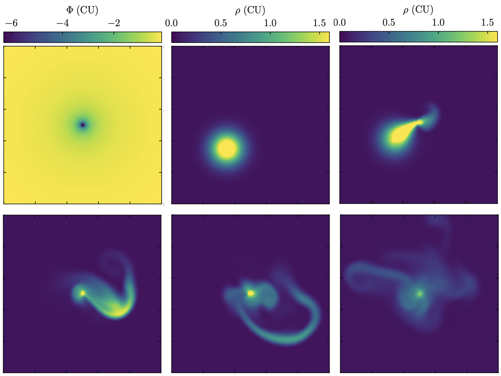
- class ulula.setups.tidal_disruption.SetupTidalDisruption(unit_l=1.0, unit_t=1.0, unit_m=1.0)
Gravitational tidal disruption
The gravitational potential in the domain represents a point mass at the center. A gas blob moves past the point mass and is tidally disrupted. This setup demonstrates
Fixed-potential gravity
Behavior at strong potential gradients.
- Parameters:
- unit_l: float
Code unit for length in units of centimeters.
- unit_t: float
Code unit for time in units of seconds.
- unit_m: float
Code unit for mass in units of gram.
- __init__(unit_l=1.0, unit_t=1.0, unit_m=1.0)
Keplerian disk
The following image shows the Keplerian disk setup as instabilities are developing:
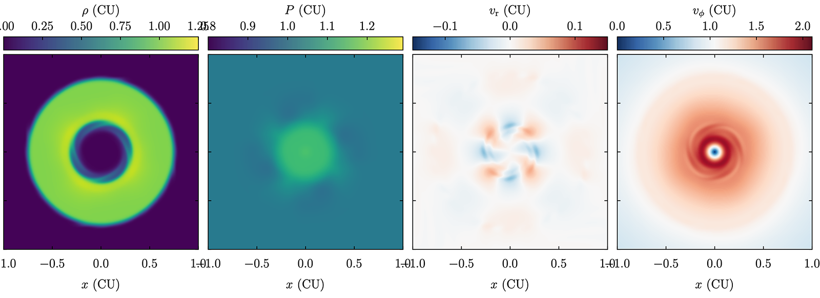
- class ulula.setups.keplerian_disk.SetupKeplerianDisk(soft_edges=False, edge_delta_r=0.02, unit_l=1.0, unit_t=1.0, unit_m=1.0)
Keplerian rotating disk
In this classic test, a dense gas disk is rotating with a velocity that balances a point-mass potential via the centrifugal force. This is a notoriously difficult test for Eulerian (grid) codes. To avoid the singularity at the center, the potential is softened. The boundary conditions are set to the same rotation speed and fluid state as the initial conditions. This setup demonstrates:
Rotating boundary conditions
Fixed potential with softening
Conservation of angular momentum.
- Parameters:
- soft_edges: bool
If True, soften the edges of the disk in density with a Gaussian profile of width
edge_delta_r.- edge_delta_r: float
See
soft_edges.- unit_l: float
Code unit for length in units of centimeters.
- unit_t: float
Code unit for time in units of seconds.
- unit_m: float
Code unit for mass in units of gram.
- __init__(soft_edges=False, edge_delta_r=0.02, unit_l=1.0, unit_t=1.0, unit_m=1.0)
Merger
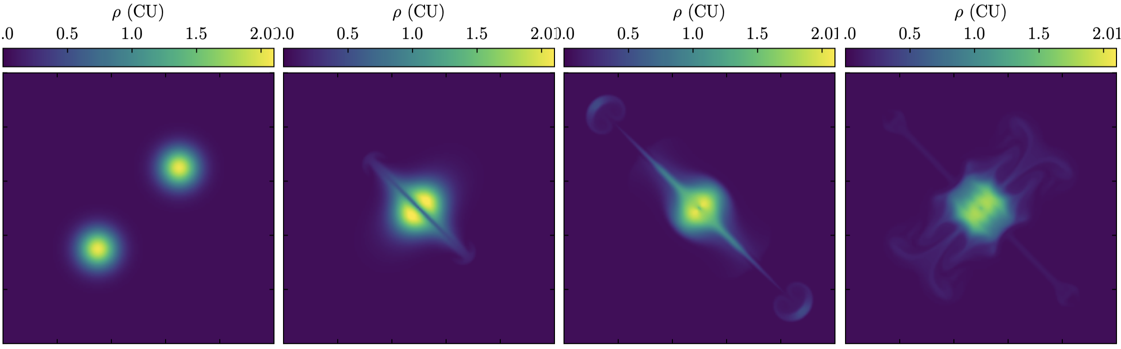
The following image shows the evolution of density in the merger setup:
- class ulula.setups.merger.SetupMerger(unit_l=1.0, unit_t=1.0, unit_m=1.0)
Merger of two gas blobs
This setup demonstrates Poisson gravity in a periodic domain. Two gas blobs with Gaussian density profiles are set along the diagonal of the domain and fall towards each other. The interplay of gravity and pressure creates complex (but symmetric) patterns, and the blobs eventually merging into a single blob. This test demonstrates:
Poisson gravity in 2D
Preservation of symmetry
- Parameters:
- unit_l: float
Code unit for length in units of centimeters.
- unit_t: float
Code unit for time in units of seconds.
- unit_m: float
Code unit for mass in units of gram.
- __init__(unit_l=1.0, unit_t=1.0, unit_m=1.0)